Probability Theory For Machine Learning (Part 1)

Data is one of the essential ingredients for building the best machine learning models. The more you know about the data, the better your machine learning model will be, as you will be able to depict the reason behind your model's performance. Probability is one of the most important mathematical tools that help in understanding different data patterns. Famous algorithms in machine learning like Naive Bayes are completely derived from the probability theory. Hence, knowing probability basics will always be considered to be the best to start the ML journey.

In this article, we will not be only describing the theoretical aspects of probability, but we will give you a sense of where those theoretical aspects will be used in ML. So, let’s start without any further delay.

If we have to define “probability”,

Originated from the “Games of Chance,” probability in itself is a branch of mathematics concerned about how likely it is that a proposition is true.

In a more layman manner, Probability is simply a Possibility of occurring a random event. For example, what is the possibility of having rain tomorrow? The values of probability can only lie between 0 and 1, with 0 and 1 inclusive.

If we notice carefully, every daily-life phenomenon can only be of two types:

• Deterministic: Phenomena that will always be true. For example, picking a white ball from a bag of white balls. Here probability will be either 0 or 1.

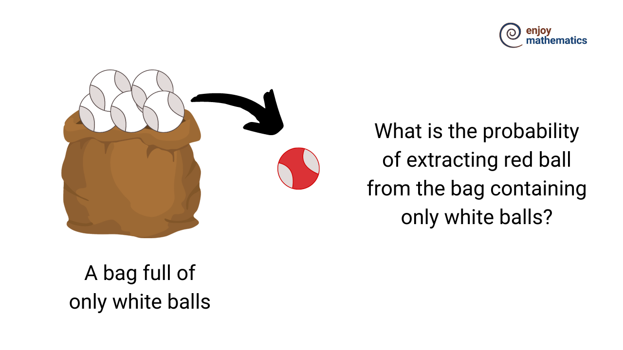
• Indeterministic: Phenomena for which we are not sure. For example, if a fair dice is rolled, the probability of the number being 1 is indeterministic.

Relationship between events

There are two famous terms when we define the relationship between events from the same experiment. 

1. Exclusive: If the two events can never happen at the same time. For example, flipping a fair coin once can not lead to the scenario where Heads and Tails both come up.
2. Exhaustive: If the probability of happening different events collectively captures all possible events that can happen. For example, in an experiment of flipping the coin, the probability of getting Heads and the probability of getting Tails capture all possible outcomes from that experiment.

IGotAnOffer

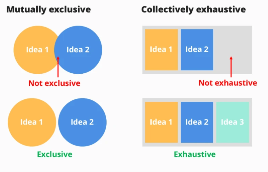
Mathematically, probability can be defined as:
If a random experiment has n > 0 mutually exclusive, exhaustive, and equally likely events and, if out of this n, m such events are favorable ( m ≥ 0 and n ≥ m), then the probability of occurrence of any event E can be defined as

Some common terms:

• Random experiment: Experiments or processes where the outcome is not predicted with certainty, like throwing a die (we can get any one of these 1,2,3,4,5,6).
• Trails and Events: The occurrence of any event in a random experiment is a trial and, the outcomes of the random experiment are events. Throwing dice is a trial, and if it shows any number from 1 to 6, then that number is an event.
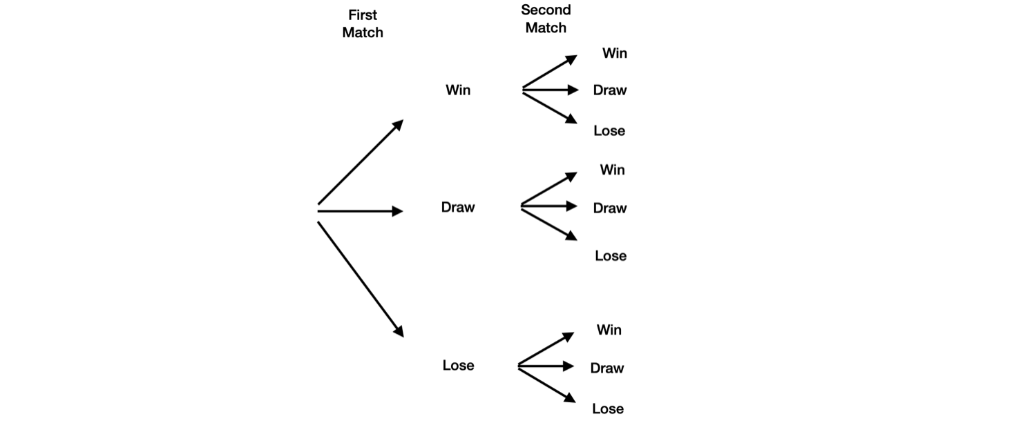
• Multiplication Rule: Ifan experiment has multiple components and1st component has K1 possible outcomes, the 2nd component has K2 possible outcomes, . . . , and the Kth component has Kr possible outcomes, then overall there are K1*K2 *. . . *Kr possibilities for the whole experiment.

• Sampling: A technique in which samples are chosen from a larger population. The sample will be considered as a probability sample if it has been chosen from a random selection.
• Exhaustive Event: Total number of all possible events of a random experiment. Like the tossing of a die once has 6 exhaustive events. If the die is tossed for n number of times, there will be 6^n exhaustive events.
• Mutually Exclusive Events: Events where the probability of any event's occurrence does not depend upon the probability of occurrence of another event in the same or different trails. Like the occurrence of 5 and 6 when two dies are rolled simultaneously.
• Equally likely events: The events where one cannot expect in preference of another event in a random experiment like rolling of a fair die twice.
• Independent Events: The eventsA and B are said to be independent events if the probability of occurrence of A doesn’t depend upon the probability of occurrence of B. Mathematically, we can say that independent events must follow:

• Conditional Independent Events: Based on some event C, A & B events are conditional independent if P(A Ո B | C) = P(A | C) P(B | C). Conditional independence does not imply independence, and independence does not imply conditional independence. Try to think over this.
• De Morgan’s Law: A̅ is the complement of A, i.e., A and A̅ are exhaustive events. U is the union of events and ∩ is the intersection of events.

Some Basic results:

Let A and B are two events; A̅ is the complement of A, then.

Probability Under Statistical Independence:

Suppose two coins are to be tossed, then the probability of occurrences of the head or tail can be classified as:

1. Marginal Probability: The simple probability of occurrence of head or tail on tossing of a coin. (Simple probabilities of occurrence of any event).
2. Joint Probability: Probability of occurrence of the head with the first coin and probability of occurrence of the tail with the second coin when both the coins are tossed simultaneously. OR When a single coin is tossed consecutively, the probability of occurrence of the tail in the first chance and head in the second chance. (Probability of occurrence of joint events occurring together or in succession).
3. Conditional Probability: Probability of occurrence of a head in tossing a coin when the tail has already occurred. (Probability of occurrence of any event A when B has already occurred).

Probability under Statistical Dependence:

When the probability of one event's occurrence depends on the probability of another event's occurrence, that scenario comes under statistical dependence. 
If we have two events, A and B, then:
1. Conditional Probability is the probability of occurrence of an event A if event B has already occurred.

2. Joint Probability is the measure of two or more events happening at the same time. It can only be applied to situations where more than one observation can occur simultaneously, i.e., the probability of occurrence of event B at the same time when event A occurs.

3. Marginal Probability is obtained by summing up probabilities of all the joint events in which a simple event is involved.

Law of Total Probability

If B1, B2, …, Bn are disjoint events and their union completes the entire sample space (i.e., they are mutually exhaustive), then the probability of occurrence of an event A will be 

P (A) = P (A ∩ B1) + P (A ∩ B2) + · · · + P (A ∩ Bn)

Baye’s Theorem: 

This is one of the most famous theorems in probability and lies in the heart of the Naive Bayes algorithm in Machine Learning.

Source

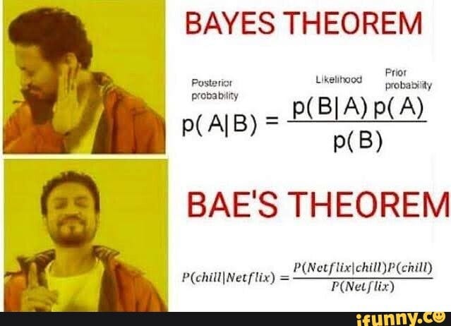
In the context of the above image,
P(chill):= Probability that you are chilling out.
P(Netflix):= Probability that you are watching Netflix.
P(chill/Netflix):= Probability that you are chilling while watching Netflix.
P(Netflix/chill):= Probability that you will watch Netflix while chilling out.

More formally, Let S be a sample space such that B1, B2, B3… Bn form the partitions of S and let A be an arbitrary event then,

𝑃(𝐵𝑖 ), 𝑖 = 1,2, …, 𝑛 are called the prior probabilities of occurrence of events.

𝑃(𝐵𝑘/A) is the posterior probability of 𝐵𝑘 when 𝐴 has already occurred.

Random Variables:

Unlike algebraic variables, where the variable in an algebraic equation is unknown and calculated, random variables take on different values based on the outcomes of any random experiment. It is just a rule that assigns a number to each possible outcome of an experiment.

Mathematically, a random variable is defined as a real function (X or Y or Z) of the elements of a sample space S to a measurable space E, i.e.,

𝑋∶𝑆 →𝐸

In more layman language,

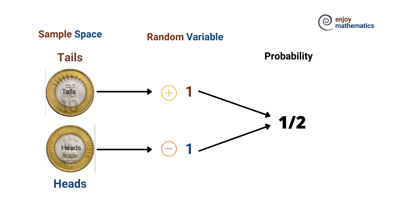
Random variables are of two types:

1. Discrete random variables: one which has finite numbers of distinct values, basically as count. Ex.- Number of times the head occurs if a coin is tossed thrice.
2. Continuous random variables: one which is defined in range. Ex.- Amount of sugar in 10ml orange juice.

That's it for this article. There are some important concepts related to probability distribution function, mathematical expectations, and famous distribution functions about which we will discuss in part 2 of the probability theory blog.

Conclusion

In this article, we discussed the basics and most commonly used terminologies in probability and machine learning. We discussed things like deterministic and indeterministic probabilities, exclusive and exhaustive events, the definition of some famous terms, marginal, joint, and conditional probabilities, the famous Baye’s theorem, and in the last, we talked about the random variables. We hope you have enjoyed the article.

Enjoy Learning! Enjoy Mathematics!